The Machine Learning Practitioner’s Guide to Reinforcement Learning: Overview of the RL Universe
Refer to doc
LIST
- Why Reinforcement Learning? Why Not Supervised Learning?
- Optimizing the Reward Function
- Supervised Learning With Labels
- Distribution Shifts
- Anatomy of an RL Algorithm
- Collecting the Data
- Off-Policy vs On-Policy
- Exploration vs Exploitation
- Why Off-Policy?
- Why On-Policy?
- Computing the Return
- Estimating the Expected Return in Model-Free Settings
- Discount Factor
- Value Functions
- N-Step Returns
- Updating the Policy
- Q-Learning
- Policy Gradients
Why Reinforcement Learning? Why Not Supervised Learning?
强化学习的最重要目标是最大化cumulative reward / return,为了达到这个目标,agent需要找到一个可以根据给定state $s$ 预测action $a$ 的policy $\pi(s)$,来最大化return
Optimizing the Reward Function
Just like we minimize a loss function using gradient descent in standard ML, can we maximize the returns using gradient ascent too? (Instead of finding the minima, gradient ascent will converge on the maxima.) Or is there a problem?
Consider a mean-squared loss for a regression problem(回归问题的均方根损失). The loss is defined by: \(L(X,Y;\theta)=\frac{1}{2}(Y-\theta^TX)^2\) Here $Y$ is the label, $X$ is the input, and $\theta$ are the weights of the neural network. The gradient of this can be easily computed.
另一方面,return由增加rewards来构造,rewards由环境的reward function生成,但是在很多场景下如model-free setting,无法知道reward function. 我们不知道这个function就无法计算梯度. So, this approach won’t work!
Supervised Learning With Labels
If the reward function is not known to us, maybe what we can do is construct our own loss function which basically penalizes惩罚 the agent if the action taken by the agent is not the one that leads to the maximum return. In this way, the action predicted by the agent becomes the prediction $\theta^TX$ and the optimal action becomes the label.
最优动作变成标签,agent预测的动作即为预测值。
For determining the optimal action at each step, we require an expert human/software. Examples of work done in this direction include Imitation Learning and Behavioural Cloning where the agent is supposed to learn using demonstrations(示范动作) by an expert (head to further reading for links on these).
However, the number of demonstrations/labeled data required for such an approach may prove to be a bottleneck for good training(充分训练的瓶颈). 人工标记是一项昂贵的业务,鉴于深度学习算法往往需要大量数据,因此收集如此多的专家标记数据可能根本不可行。另一方面,如果一个人有一个专家软件,那么人们需要想知道为什么要使用 AI 构建另一个软件来解决我们已经拥有专家软件的任务!
Furthermore, approaches that use expert trained data for supervision are often limited by the upper bound of the expertise of the expert. The policy of the expert may just be the best available at the moment, not the optimal one. We would ideally like the RL agent to discover the optimal policy (which maximizes the return).
Also, such approaches would not work for unsolved problems for which we don’t have experts.
Distribution Shifts
解决 expert-labelled 数据问题的另一个问题是分布偏移distribution shifts。让我们考虑一个专家代理玩 SeaQuest 的案例,这是一款您从海底接载潜水员的游戏。该agent的氧气来源正在耗尽,必须定期到地表重新收集氧气。
假设expert agent的策略永远不会让agent处于氧气低于 30% 的状态。因此,按照此策略收集的任何数据都不会包含氧气低于 30% 的状态。
现在想象一个agent是从使用上述专家策略创建的数据集训练的。如果受过训练的agent不完美(100% 的表现是不现实的)并且发现自己处于氧气含量约为 20% 的状态,则它可能没有经历过在这种状态下应采取的最佳行动。这种现象称为distribution shift ,可以使用下图来理解。

One famous work in imitation learning that has been used to combat distribution shifts Dagger, a link to which I have provided below. However, this approach was also marred by high data acquisition costs both in terms of money and time spent.
The Anatomy of an RL Algorithm
In RL, instead of learning using labels, the agent learns through trial and error. The agent tries out a bunch of things observing what fetches a good return and what fetches a bad return. Using various techniques, the agent comes up with a policy that is supposed to execute actions that give maximum or close to maximum returns.
RL algorithms comes in all shapes and sizes but most of them tend to follow a template which we here refer as the Anatomy of a RL algorithm.
Any RL algorithm, in general, breaks the learning process into three steps.
- Collect the data
- Estimate the return
- Improve the policy.
以上步骤会重复多次直到达到理想性能,这里没有用到 convergence收敛 这个词,因为对于很多深度强化学习算法,没有收敛的理论保证,只是它们在实践中似乎可以很好地解决各种问题。
Collecting the Data
与标准机器学习设置不同,RL 设置中没有静态数据集,我们可以反复迭代以改进我们的策略。相反我们通过与环境交互进行收集数据,The policy is run and the data is stored. 数据通常以4元组存储$⟨s_t,a_t,r_t,s_{t+1}⟩$
$s_t$ 是初始状态,$a_t$是采取的动作,$r_t$是在$s_t$下采取$a_t$所累积的reward,$s_{t+1}$是在$s_t$下采取$a_t$后转移的状态。
Off-Policy vs On-Policy
RL algorithms often alternate交替进行 between collecting data and improving the policy. The policy that we use to collect the data maybe different from the policy which we are training. This is called Off-Policy Learning.
The policy which collects the data is called the Behavioural policy, while the policy which we are training (which we plan to use using test time) is called the Target Policy.
In an alternate setting, we might use the same policy which we are training to collect the data. This is called On-Policy Learning. Here the Behavioural policy and the target policy are the same.
两者区别:
Consider we are training a target policy which gives us an estimated return for each action (consider actions to be discrete), and we have to chose the action that maximizes this estimate. In other words, we act greedily with respect the the action score.(考虑动作收益来“贪心”地做决策 \(\pi(s)={\underset {a∈A}{\operatorname {arg\,max} }}\,R_{estimate}(a)\) Here, $R_{estimate}(a)$ is the return estimate.
During the data collection phase, we chose random actions to interact with the environment, disregarding return estimates(忽视估计回报. When we update our target policy, we assume that the trajectory taken by the policy beyond $⟨s_t,a_t,r_t,s_{t+1}⟩$ would be determined by choosing actions greedily w.r.t to estimated return. In contrast, when we collect the data, we pick random actions.
Therefore, our behavioural policy is different from our training one i.e. the greedy policy. This is therefore off-policy training.
相当于收集数据的时候是随机选择动作,在更新target policy的时候,就会贪心地选择回报更高的轨迹
If we use the greedy policy for data collection as well, this would become an on-policy setting.
Exploration vs Exploitation
Apart from the credit assignment problem, this is the one of THE biggest challenge in RL; so much so that guarantees it’s own post, but I will try to give a brief overview here.
举了个例子,是要继续严格使用之前的方法,还是尝试一些新的方法。
All these scenarios are basically choices between whether we want to explore more in pursuit of new tools, or exploit the knowledge we currently have! 探索&利用
在 RL 算法的世界中,agent从探索所有behaviours开始。在适当的训练过程中,通过反复试验,它在一定程度上认识到什么有效/什么无效。
Once it gets to a decent level of performance一旦它达到了不错的表现水平,它是否应该利用它所学到的东西,随着训练的进一步发展变得更好?或者它应该探索更多以发现最大化回报的新方法。这就是exploration v/s exploitation困境的核心所在。
RL 算法必须平衡两者以确保良好的性能。最好的解决方案位于完全探索性和利用性行为的中间。有多种方式将这些行为的平衡融入到数据收集策略中。
In an off-policy setting, the data collection policy maybe totally random leading to overly exploratory behaviour. Alternatively, one can take a step according to the training policy or take a random action randomly with some probability. This is a popularly used technique in Deep RL.
p = random.random()

if p < 0.9:
	# act according to policy
else:
	# pick a random action
In on-policy settings, we can 扰动 perturb **the actions using some noise, or predict the parameters of a probability distribution and **sample from it to determine what actions to take.
Why Off-Policy?
The biggest advantage of off policy learning that it helps us with exploration.
The target policy can turn very exploitative in nature, not explore the environment well enough and settle for a sub-optimal policy. A data collection policy that is exploratory in nature will deliver diverse states from the environment to the training policy. For this reason, the behavioural policy is also called the exploratory policy.
Additionally, off-policy learning allows the agent to use data from older iterations whereas for on-policy learning, new data has to be collected every iteration. However, if the data collection operation is expensive, then on-policy may increase computational time of the training process.
on-policy每次都要重新收集数据,开销会很大
Why On-Policy?
If off-policy learning is so great at encouraging exploration, why do we even want to use on-policy learning? Well, the reason has to do a bit with the mathematics of how the policy is updated (step 3).
With off-policy updates, we are basically updating the behaviour of the target policy using trajectories generated by another policy. Given similar set of initial states and action, our target policy could have led to different trajectories and returns. If these diverge too much, the updates can modify the policies in unintended ways.(可能会导致意外的结果
It is for this reason we don’t always go for off-policy learning. Even when we do, the updates only work well when the difference between two policies ain’t very large, therefore, we sync our target and behavioural polices periodically(周期性的同步) and use techniques like importance sampling when making off-policy learning updates.
Computing the Return
The central goal of Reinforcement Learning is to maximise the expected cumulative reward, or simply the return . The word expected basically factors in the possible stochastic nature of policy as well as the environment.(预期一词主要是policy和环境可能的随机性因素。
When we are dealing with cases where the environments are episodic有间断的 in nature (i.e. an agent’s life terminates eventually. Like a game such as Mario, where the agent can finish the game, or die by falling / getting bitten), the return is termed as a finite-horizon return. In case where are dealing with continuing连续的 environments (no terminal state), the return is termed as an infinite-horizon return.
Let us only consider episodic environments. Our policy might be stochastic, i.e. given a state $s$, it may take different trajectories $\pi$ to the terminal state, $s_T$.
We can define a probability distribution over these trajectories using:
- Policy (which gives us the probabilities of various actions), and
- The state transition function of the environment (which gives us the distribution of future states given state and action).
The probability of any trajectory starting from an initial state $s_1$ and ending in a terminal state $s_T$ is given by

Once we have the probability distribution over trajectories, we can compute the expected return over all possible trajectories as follows.

It is this quantity that RL algorithms are designed to maximise.
Note that it is very easy to get confused between reward and return. The environment provides the agent a reward for every single step whereas return is the sum of these individual rewards.
reward是单步奖励,return是总奖励
We can define return $G_t$ at the time $t$ as the sum of rewards from that time. \(G_t=\sum^{T}_{t}{r(s_t, a_t)}\) Generally, when we talk about maximising the expected return as an objective of solving the RL task, we talk about maximising $R_1$ i.e. the return from the initial state.
Mathematically, we optimise the algorithms to maximise every $R_t$. If the algorithm is able to maximise every $R_t$, then $R_1$ gets automatically maximised. Conversely, it’s absurd to try maximise$R_{1…t-1}$ using action taken at time $t$. The policy can’t alter actions taken previously.
To differentiate $R_1$ return from the general return $R_t$, we will call the former the test return and latter, just the return.

The return for any state is sum of cumulative reward from that state to the terminal state.
Estimating The Expected Return In Model-free Settings
Recall from the last post that a lot of times we try to directly learn from experiences and we have no access to state transition function. Such settings are a part of Model-free RL. In other cases, the state space may be so large that computing all the trajectories is intractable.
In such cases, we basically run the policy multiple times and average the individual returns to get an estimate value of return. The following expression estimates the expected return. \(\frac{1}{N}\sum^{N}_{i}\sum^{T}_{t}{r(s_{i,t}, a_{i,t})}\) where $N$ is the number of runs, and ${r(s_{i,t}, a_{i,t})}$ is the reward got obtained at time $t$ in the $i^{th}$ run
The more the number of runs we do, the more accurate will our estimate be.
Discount Factor
There are a couple of problems with the above formulation for the expected return.
- In the case of continuing tasks where there is no terminal state, the expected return is an infinite sum. Mathematically, this sum may not converge with an arbitrary reward structure.
- Even in the finite horizon case, the return for a trajectory consists of all the rewards starting a state, say, $s$ all the way up the terminal state $s_T$. We weigh all the rewards equally, irrespective of whether they occur sooner or much later. That is quite unlike how things work in real life.
The second point basically asks the question “Is it necessary to add all the future rewards while calculating the return?” Maybe we can do with only the next 10 or 100? That will also solve the problem arising with continuing tasks since we don’t have to worry about infinite sums.
Consider you are trying to teach a car how to drive through RL. The car gets a reward between 0 and 1 for every time step depending upon how fast it’s going. The episode terminates once we have clocked 10 minutes of driving or earlier in case of collision.
Imagine the car gets too close to a vehicle and must slow down to avoid a collision and termination of the episode. Note that collision might still be a few time steps away. Therefore, until the collision happens, we will still be getting rewards for high speed before the car crashes. If we just consider only immediate or the 3 immediate returns for the reward, then we will be getting a high return even when we are on the collision course!
Suppose, the 10-minute episode is divided into 100 time steps. The car goes at full speed till 80 time steps and 0 afterward since it collides at the 80th time step. Ideally, it should have slowed down to avoid the collision.
Using Instantaneous Rewards as Return.

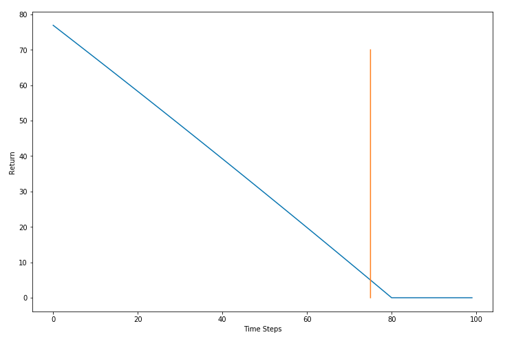
Let’s now use the future three rewards to compute the return.
Using three future rewards as return.
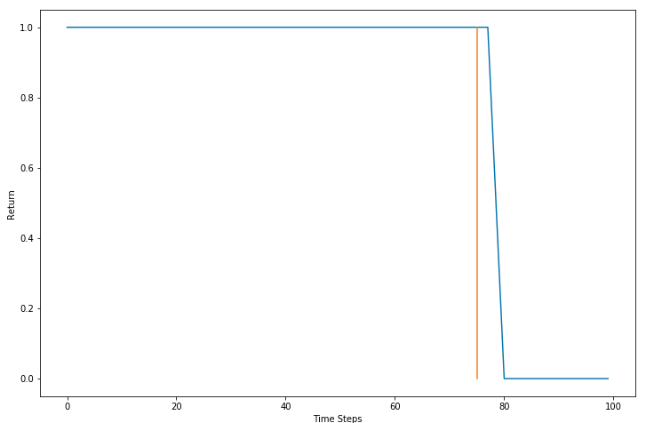
The orange line represents the 75 time-step mark. The vehicle should at least start to slow down here. In other words, the return should be less so such behaviors (speed on a collision path) are discouraged. The return starts to fall only after the 78th time step when it’s too late to stop. The return for speeding at the 75th time step should be less too.
We want returns that incentivize foresight. Maybe we should add more future rewards to compute our returns. (希望有先见之明—-加入未来rewards)
What if we add all the future returns like in the original formulation. With that, our return keeps falling as we move forward, even during time steps 1-50. Note that actions taken during T = 1-50 have little to no effect on the actions that led to the collision at T = 80.
Adding all future rewards to the return
最好介于两者之间————引入$\gamma$, 重写 expected return. \(\frac{1}{N}\sum^{N}_{i}\sum^{T}_{t}\gamma^{t-t' } { r(s_{i,t}, a_{i,t})}\) Here is how the discounted return $G_1$ looks like. \(G_1=r_1+\gamma r_2+\gamma^2r_3+……\) This is often termed as discounted expected return. $\gamma$ is called the Discount Factor
$\gamma$ lets us control how far we are looking into the future when it comes to using rewards to compute our return. A higher value of $\gamma$ will have us look further into the future. The value of $\gamma$ is between 0 and 1. The weightage of the rewards fall exponentially(指数下降) with each time step. Popular values used in practice are 0.9, 0.99 and 0.999. The following graph shows how γγ effects the return for our car example.
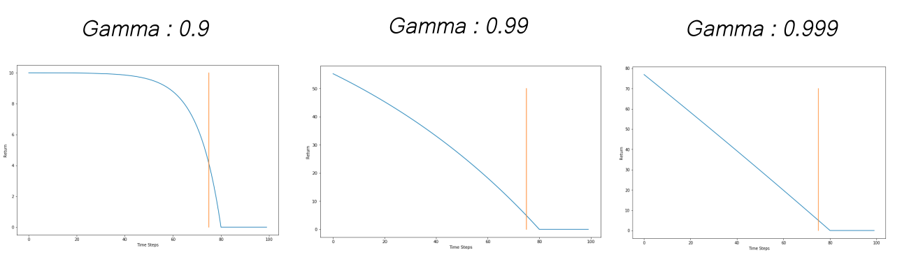
A higher $\gamma$ means that the the agent looks much further into the future. Conversely, the effect of collision on the return is seen on much earlier time steps with a higher $\gamma$
Under reasonable assumptions, discounted infinite sums can be shown to converge, which makes them useful in cases of continuing environments with no terminal state.
Value Functions
While we can define compute the discounted returns in the way mentioned above, here is a catch (存在问题). Computing such a return for any state will require you to complete the episode first or carry out a large number of steps before you can compute the return. 需要完成整个过程才能进行计算
Another way to compute the returns is to come up with a function, that takes the state $s$ and the policy $π$ as the input and estimates the value of the discounted return directly, rather than us having to add up future rewards.
The value function for a policy $π$ is written as $V^π(s)$. Its value is equal to the expected return if we were to follow the policy $π$ starting from state $s$. In RL literature, the following notation is used to describe the value function. \(V^\pi(s)=\mathbb{E}[G_t|S_t=s]\) Note that we don’t write $G_t$ as a function of the state and the policy. This is because we treat $G_t$ just as sum of rewards returned from the environment. We have no clue (in model-free settings) how these rewards are computed.
However, Vπ(s)Vπ(s) is a function that we predict ourselves using some estimator like a neural network. There, it’s written as a function in the notation.
A slight modification of the value function is the Q-Function which estimates the expected discounted return if we take an action $a$ in the state $s$ under policy $π$. \(Q^\pi(s,a)=\mathbb{E}[G_t|S_t=s,A_t=a]\) The policy that maximises the value function for all states is termed as the optimal policy.
There are quite a few ways how value functions are learned in RL. If we are in a model-based RL environment and the state space is not prohibitively large, then we can learn value functions through dynamic programming. These methods use recursive formulations of value functions, known as the Bellman Equations to learn them. We will cover Bellman Equations in-depth later in a post on Value Function Learning. (递归去计算-贝尔曼等式
Bellman equation decomposes the value function into two parts, the immediate reward plus the discounted future values.
This equation simplifies the computation of the value function, such that rather than summing over multiple time steps, we can find the optimal solution of a complex problem by breaking it down into simpler, recursive subproblems and finding their optimal solutions.


In the case where the state space is too large, or we are in a model-free setting, we can estimate the value function using supervised learning where labels are estimated by averaging many returns.
N-Step Returns
We can mix returns and value functions to arrive at what are called n-step returns. \(G_t^n=r_t+\gamma r_{t+1}+……+\gamma^{n-1}r_{t+n-1}+\gamma^3V(s_{t+n})\) In literature, using the value functions for computing the rest of the return (that come after n-steps) is also called as Bootstrapping.
Updating the Policy
In the third part, we update the policy so that it takes actions which maximise the Discounted Expected Reward (DER)
There are a couple of popular ways to learn the optimal policies in Deep RL. Both of these approaches contain objectives that can be optimised using Backpropagation.
Q-Learning
In Q-Learning, we learn a Q-function and pick actions by acting greedy w.r.t to the Q-values for each action. We optimise a loss with an aim to learn the Q-function.
Policy Gradient
We can also maximise the expected return by performing gradient ascent on it. The gradient is called the policy gradient.
In this approach, we directly modify the policy so that actions that led to more rewards in experience collected are made more likely, while the actions that led to bad rewards are made less likely in the probability distribution of the policy.
Another class for algorithms called Actor-Critic algorithms combines Q-Learning and policy gradients .
More
Important Sampling
In RL, importance sampling estimates the value functions for a policy π with samples collected previously from an older policy π’. In simple term, calculating the total rewards of taking an action is very expensive. However, if the new action is relatively close to the old one, importance sampling allows us to calculate the new rewards based on the old calculation.
In specific, with the Monte Carlo method in RL, whenever we update the policy θ, we need to collect a completely new trajectory to calculate the expected rewards.

A trajectory can be hundreds in steps and it is awfully inefficient for one single update. With importance sampling, we just reuse the old samples to recalculate the total rewards. However, when the current policy diverges from the old policy too much, the accuracy decreases. Therefore, we do need to resync both policies regularly.
In other situations. we use importance sampling to rewrite the Policy Gradient equation and use them to create new solutions.

For example, we can reposition our optimization with constraints of not going too far in changing the policy. We formalize a trust-region concept which we believe the approximation is still accurate enough for those new policies within the region.

By not making too aggressive moves, we have better assurance that we don’t make bad changes that spoils the training progress. As we keep improving the policy, we locate the optimal solution.
主要是找一个more tractable distribution进行采样